Modeling Linear PDE Systems with Probabilistic Machine Learning
Bogdan Raiță
Department of Mathematics and Statistics
Georgetown University
With many, many contributions by Marc Härkönen, Markus Lange-Hegermann, Jianlei Huang, and Xin Li
Differential Equations and Data: Why?
- Combine expert knowledge and data.
- Want intepretable and reliable models.
- Focus on (irregularly spaced) data rather than IC/BC.
- Numerical simulations might be computationally too costly.
Example
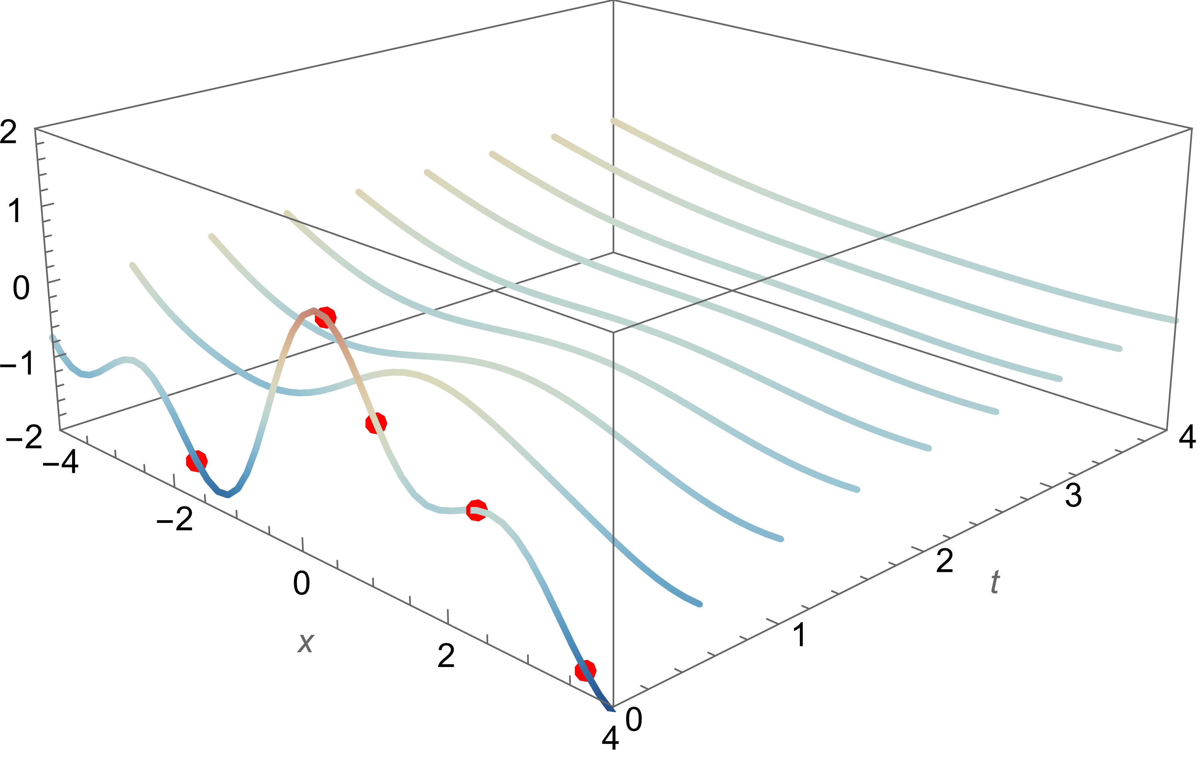
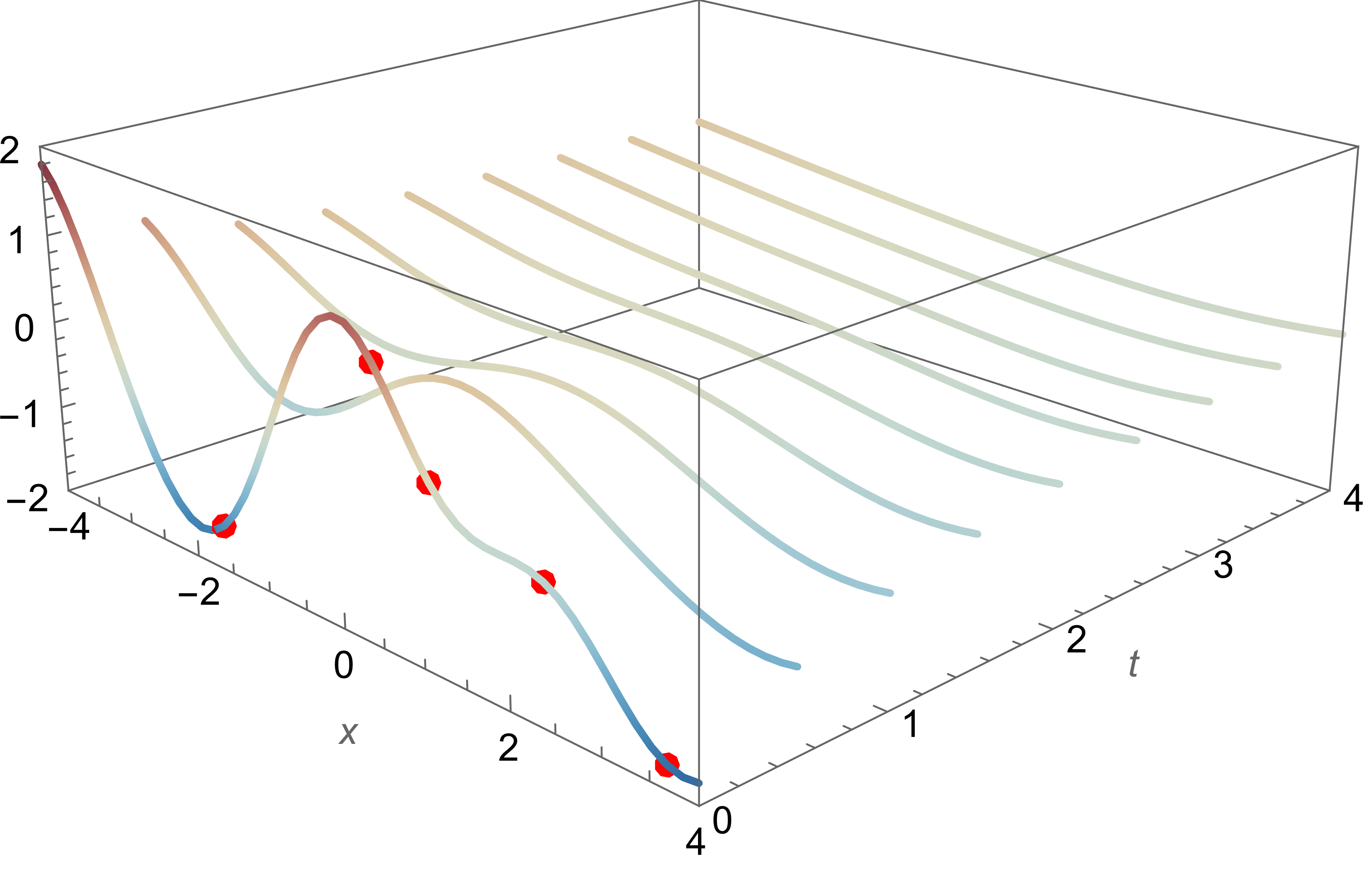
Damped spring-mass system
\[\frac{\mathrm{d}^2y}{\mathrm{d}t^2} + 2 \frac{\mathrm{d}y}{\mathrm{d}t} + 10y = 0\] Sample 5 noisy points
Example
Neural Network
- ⚠️ ~300,000 parameters
- ✅ Fast convergence
- ❌ Bad inter/extrapolation
Example
Physics Informed Neural Network
- ✅ Good interpolation
- ✅ Fast inference
- ⚠️ ~300,000 parameters
- ⚠️ Requires extra points
- ⚠️ Not an exact solution
- ❌ Slow convergence
- ❌ Hard to optimize
A more constrained approach
How to solve? \[\frac{\mathrm{d}^2y}{\mathrm{d}t^2} + 2 \frac{\mathrm{d}y}{\mathrm{d}t} + 10y = 0\]
Algebraic preprocessing: characteristic frequencies \[z^2 + 2z + 10 = 0 \Rightarrow z = -1 \pm 3\sqrt{-1}\]
Solution Space \[y(t) = (\textcolor{#b51963}{c_1} \cdot e^{-t} \cos 3t + \textcolor{#b51963}{c_2} \cdot e^{-t} \sin 3t)\]
Gaussian process prior \[Y(t) \sim (\textcolor{#b51963}{C_1} \cdot e^{-t} \cos 3t + \textcolor{#b51963}{C_2} \cdot e^{-t} \sin 3t) + \textcolor{#b51963}{\epsilon}\] where \[ \textcolor{#b51963}{C_1 \sim \mathcal{N}(0, \sigma_1)}, \textcolor{#b51963}{C_2 \sim \mathcal{N}(0, \sigma_2)}, \textcolor{#b51963}{\epsilon \sim \mathcal{N}(0, \sigma_0)} \]
Algebra: determine suitable frequencies
Stochastic: weigh frequencies
Gaussian Process
(or ridge regression)
- ✅ 3 parameters
- ✅ Fast convergence
- ✅ Good inter/extrapolation
- ✅ Exact solution
- ✅ No extra points
Overview
| EPGP (ours) | S-EPGP(ours) | Vanilla PINN | Vanilla Num. Solver | |
|---|---|---|---|---|
| Differential equations | linear, c.c. | linear, c.c. | any | well-posed |
| Additional Information | data | data | data | IC/BC |
| Evaluation time | $\approx$ data | $\approx$ sparsity | neural net | mediocre |
| Solutions? | yes | yes | approx. near data | yes |
| Prerequisites | integral | - | - | - |
| Sampling | yes | yes | no | not applicable |
Another ODE example
How to solve? \[\frac{\mathrm{d}^4y}{\mathrm{d}t^4} + 2 \frac{\mathrm{d}^2y}{\mathrm{d}t^2} + y = 0\]
Another ODE example
How to solve? \[\frac{\mathrm{d}^4y}{\mathrm{d}t^4} + 2 \frac{\mathrm{d}^2y}{\mathrm{d}t^2} + y = 0\]
Algebraic preprocessing: characteristic frequencies \[z^4 + 2z^2 + 1 = 0 \Rightarrow z = \pm i\text{ with multiplicity 2}\]
Another ODE example
How to solve? \[\frac{\mathrm{d}^4y}{\mathrm{d}t^4} + 2 \frac{\mathrm{d}^2y}{\mathrm{d}t^2} + y = 0\]
Algebraic preprocessing: characteristic frequencies \[z^4 + 2z^2 + 1 = 0 \Rightarrow z = \pm i\text{ with multiplicity 2}\]
Solution Space \[y(t) = \textcolor{#b51963}{c_1}\textcolor{#0073e6}{t}e^{\textcolor{#0073e6}{-i}t} + \textcolor{#b51963}{c_2}e^{\textcolor{#0073e6}{-i}t}+\textcolor{#b51963}{c_3}\textcolor{#0073e6}{t}e^{\textcolor{#0073e6}{i}t}+\textcolor{#b51963}{c_4}e^{\textcolor{#0073e6}{i}t}\]
Gaussian process prior \[Y(t) \sim \textcolor{#b51963}{C_1}\textcolor{#0073e6}{t}e^{\textcolor{#0073e6}{-i}t} + \textcolor{#b51963}{C_2}e^{\textcolor{#0073e6}{-i}t}+\textcolor{#b51963}{C_3}\textcolor{#0073e6}{t}e^{\textcolor{#0073e6}{i}t}+\textcolor{#b51963}{C_4}e^{\textcolor{#0073e6}{i}t} + \textcolor{#b51963}{\epsilon}\] where \[ \textcolor{#b51963}{C_j \sim \mathcal{N}(0, \sigma_j)}, \textcolor{#b51963}{\epsilon \sim \mathcal{N}(0, \sigma_0)} \]
Principle for ODEs
How to solve? \[\sum_{j=0}^k \alpha_j\frac{\mathrm d^jy}{\mathrm d t^j} = 0\]
Principle for ODEs
How to solve? \[\sum_{j=0}^k \alpha_j\frac{\mathrm d^jy}{\mathrm d t^j} = 0\]
Algebraic preprocessing: characteristic frequencies \[\sum_{j=0}^k \alpha_jz^j=0 \Rightarrow z\in V = \text{ complex roots with multiplicities}\]
Principle for ODEs
How to solve? \[\sum_{j=0}^k \alpha_j\frac{\mathrm d^jy}{\mathrm d t^j} = 0\]
Algebraic preprocessing: characteristic frequencies \[\sum_{j=0}^k \alpha_jz^k=0 \Rightarrow z\in V = \text{ complex roots with multiplicities}\]
Solution Space \[y(t) = \sum_{\textcolor{#0073e6}{z}\in V}\sum_{\text{multipliers for z}}\textcolor{#b51963}{c_{h}}\textcolor{#0073e6}{B_h(t)}e^{\textcolor{#0073e6}{z}t} \]
Principle for ODEs:
All solutions are linear combination of exponential-polynomial solutions.
Fourier & Heat Equation
\[\frac{\partial T}{\partial t}-\frac{\partial^2 T}{\partial x^2}=0\]
Fourier & Heat Equation
\[\frac{\partial T}{\partial t}-\frac{\partial^2 T}{\partial x^2}=0\]
Fourier (1807):
- Noticed that $T_z(x,t)=e^{\textcolor{#0073e6}{-z^2}t+\textcolor{#0073e6}{iz}x}=e^{-z^2t}(\cos zx+i\sin zx)$ are solutions.
- Noticed linearity: $T^c(x,z)=\sum_{z=-N}^N \textcolor{#b51963}{c_z}e^{\textcolor{#0073e6}{-z^2}t+\textcolor{#0073e6}{iz}x}$ are solutions.
- Postulated density: All solutions $T$ can be approximated with solutions $T^c$.
- Solved from initial condition: If $T(x,0)=g(x)$ and $T\approx T^c$ then \[g(x)= \sum_{z\in\mathbb Z} \textcolor{#b51963}{c_z}e^{\textcolor{#0073e6}{iz}x}.\]
- Invented Fourier series.
Our goals
- Use additional knowledge of linear PDE systems with constant coefficients.
- Construct a computationally nice probabily distribution on such PDE systems.
- Restricting to this important special case allows more suitable methods.
- Introduce two such methods: EPGP and S-EPGP.
Principle for PDEs
All solutions are linear combination of exponential-polynomial solutions up to approximation.
Let $A \in R^{\ell' \times {\ell}}$ for $R=\R[\partial]$ where $\partial=(\partial_{x_1},\ldots,\partial_{x_n})$.
Want to solve $A(\partial)f=0$ for $f=(f_1,f_2,\ldots,f_\ell)\in \mathcal F^\ell$,
where $\mathcal F$ is a space of functions,
e.g. $\mathcal F=C^\infty(\Omega)$.
Thus $\mathcal F$ is a left $R$-module under the action of differentiation.
Principle for PDEs
All solutions are linear combination of exponential-polynomial solutions up to approximation.
Let $A \in R^{\ell' \times {\ell}}$ for $R=\R[\partial]$ where $\partial=(\partial_{x_1},\ldots,\partial_{x_n})$.
Want to solve $Af=0$ for $f=(f_1,f_2,\ldots,f_\ell)\in \mathcal F^\ell$, where $\mathcal F$ is a space of functions, e.g. $\mathcal F=C^\infty(\Omega)$.
Thus $\mathcal F$ is a left $R$-module under the action of differentiation.
Algebraic preprocessing: characteristic frequencies \[\ker A(z)=\{0\} \Rightarrow z\in V = \text{ characteristic variety}\]
Principle for PDEs
All solutions are linear combination of exponential-polynomial solutions up to approximation.
Let $A \in R^{\ell' \times {\ell}}$ for $R=\R[\partial]$ where $\partial=(\partial_{x_1},\ldots,\partial_{x_n})$.
Want to solve $A(\partial)f=0$ for $f=(f_1,f_2,\ldots,f_\ell)\in \mathcal F^\ell$, where $\mathcal F$ is a space of functions, e.g. $\mathcal F=C^\infty(\Omega)$.
Thus $\mathcal F$ is a left $R$-module under the action of differentiation.
Algebraic preprocessing: characteristic frequencies \[\ker A(z)=\{0\} \Rightarrow z\in V = \text{ characteristic variety}\]
Solution Space is the closure of \[f(x) = \sum_{j=1}^M\sum_{h=1}^m\textcolor{#b51963}{c_{j}}\textcolor{#0073e6}{B_h(x,z_j)}e^{\textcolor{#0073e6}{z_j}\cdot x} \] where $\textcolor{#0073e6}{z_j}\in V$.
This is the FUNDAMENTAL PRINCIPLE of Ehrenpreis-Palamodov ('70).
Fundamental Principle for PDEs
Explain Ehrenpreis-Palamodov in more detail:
Let $A \in R^{\ell' \times {\ell}}$ for $R=\mathbb{C}[\partial_{x_1},\ldots,\partial_{x_n}]$, $\Omega \subseteq \R^n$ be convex open, and $\mathcal F=C^\infty(\Omega)$. Then \[ \begin{align*} \ker_{\mathcal F}A=\{f\in \mathcal F^\ell\colon A(\partial) f=0 \}\simeq \dfrac{R^\ell}{\mathrm{im}_{R}A^\top}. \end{align*} \] Primary decomposition: $\mathrm{im}_R A^\top=\bigcap_{i=1}^s \mathrm{im}_R A_i^\top$ yields $\ker_{\mathcal F}A=\sum_{i=1}^s \ker_{\mathcal F}A_i$. There exist
- irreducible characteristic varieties $\textcolor{#0073e6}{\{V_1,\dotsc,V_s\}}$ and
- Noetherian multipliers $\textcolor{#0073e6}{\{B_{i,1}(x, z), \dotsc, B_{i,m_i}(x,z)\}_{i=1,\dotsc,s}}\subset\mathbb C[z,x]^\ell$.
Recent work: Cid-Ruiz-Homs-Sturmfels '21, Chen-Cid-Ruiz-Härkönen-Krone-Leykin '21.
Old work: Palamodov, Ehrenpreis '70, Hörmander '73, Björk '79, Eisenbud-Huneke-Vasconcelos '92.
Fundamental Principle for PDEs
Explain Ehrenpreis-Palamodov in more detail:
Let $A \in R^{\ell' \times {\ell}}$ for $R=\R[\partial_{x_1},\ldots,\partial_{x_n}]$ and let $\Omega \subseteq \R^n$ be a convex, open set. There exist
- irreducible characteristic varieties $\textcolor{#0073e6}{\{V_1,\dotsc,V_s\}}$ and
- $\ell\times1$ polynomials $\textcolor{#0073e6}{\{B_{i,1}(x, z), \dotsc, B_{i,m_i}(x,z)\}_{i=1,\dotsc,s}}$ in $2n$ variables,
such that any smooth solution $f \colon \Omega \to \R^{\ell}$ to the equation $A(\partial)f = 0$ can be approximated by \[ \begin{align*} f(x) &= \sum_{i=1}^s \sum_{j=1}^{m_i}\sum_h \textcolor{#b51963}{c_h^{ij}} \textcolor{#0073e6}{B_{i,j}}(x, \textcolor{#0073e6}{z^{ij}_h}) e^{\langle x, \textcolor{#0073e6}{z^{ij}_h} \rangle} \end{align*} \] where $\textcolor{#0073e6}{z^{ij}_h\in V_i}$. This is a NONLINEAR FOURIER SERIES with frequencies NOT from a lattice.
Fundamental Principle for PDEs
Explain Ehrenpreis-Palamodov in more detail:
Let $A \in R^{\ell' \times {\ell}}$ for $R=\R[\partial_{x_1},\ldots,\partial_{x_n}]$ and let $\Omega \subseteq \R^n$ be a convex, open set. There exist
- irreducible characteristic varieties $\textcolor{#0073e6}{\{V_1,\dotsc,V_s\}}$ and
- $\ell\times1$ polynomials $\textcolor{#0073e6}{\{B_{i,1}(x, z), \dotsc, B_{i,m_i}(x,z)\}_{i=1,\dotsc,s}}$ in $2n$ variables,
such that any smooth solution $f \colon \Omega \to \R^{\ell}$ to the equation $A(\partial)f = 0$ can be written as \[ \begin{align*} f(x) &= \sum_{i=1}^s \sum_{j=1}^{m_i}\int_{\textcolor{#0073e6}{V_i}} \textcolor{#0073e6}{B_{i,j}}(x, {z}) e^{\langle x, {z} \rangle}\mathrm{d\,} \textcolor{#b51963}{\mu_{i,j}}(z). \end{align*} \] This is a COMPLEX FOURIER TRANSFORM of a SINGULAR COMPLEX MEASURE.
S-EPGP
Sparse version of EPGP.
- Define a GP prior with realizations of the form \[ \begin{align*} f(x) = \sum_{j=1}^m \sum_{i=1}^r \textcolor{#b51963}{C_{i,j}} \textcolor{#0073e6}{B_j}(x, \textcolor{#0073e6}{z_{i,j}}) e^{\langle x, \textcolor{#0073e6}{z_{i,j}} \rangle} =: \textcolor{#b51963}{C^T}\cdot \textcolor{#0073e6}{\phi(x)}, \end{align*} \]
- Turn $f(x)$ into a GP: $\textcolor{#b51963}{C_{i,j} \sim \mathcal{N}\left(0, \Sigma\right)}$ for $\textcolor{#b51963}{\Sigma=\operatorname{diag}(\sigma_{i}^2)}$
S-EPGP
Sparse version of EPGP. Suitable, when integration is not possible.
- Define a GP prior with realizations of the form \[ \begin{align*} f(x) = \sum_{j=1}^m \sum_{i=1}^r \textcolor{#b51963}{C_{i,j}} \textcolor{#0073e6}{B_j}(x, \textcolor{#0073e6}{z_{i,j}}) e^{\langle x, \textcolor{#0073e6}{z_{i,j}} \rangle} =: \textcolor{#b51963}{C^T}\cdot \textcolor{#0073e6}{\phi(x)}, \end{align*} \]
- Turn $f(x)$ into a GP: $\textcolor{#b51963}{C_{i,j} \sim \mathcal{N}\left(0, \Sigma\right)}$ for $\textcolor{#b51963}{\Sigma=\operatorname{diag}(\sigma_{i}^2)}$
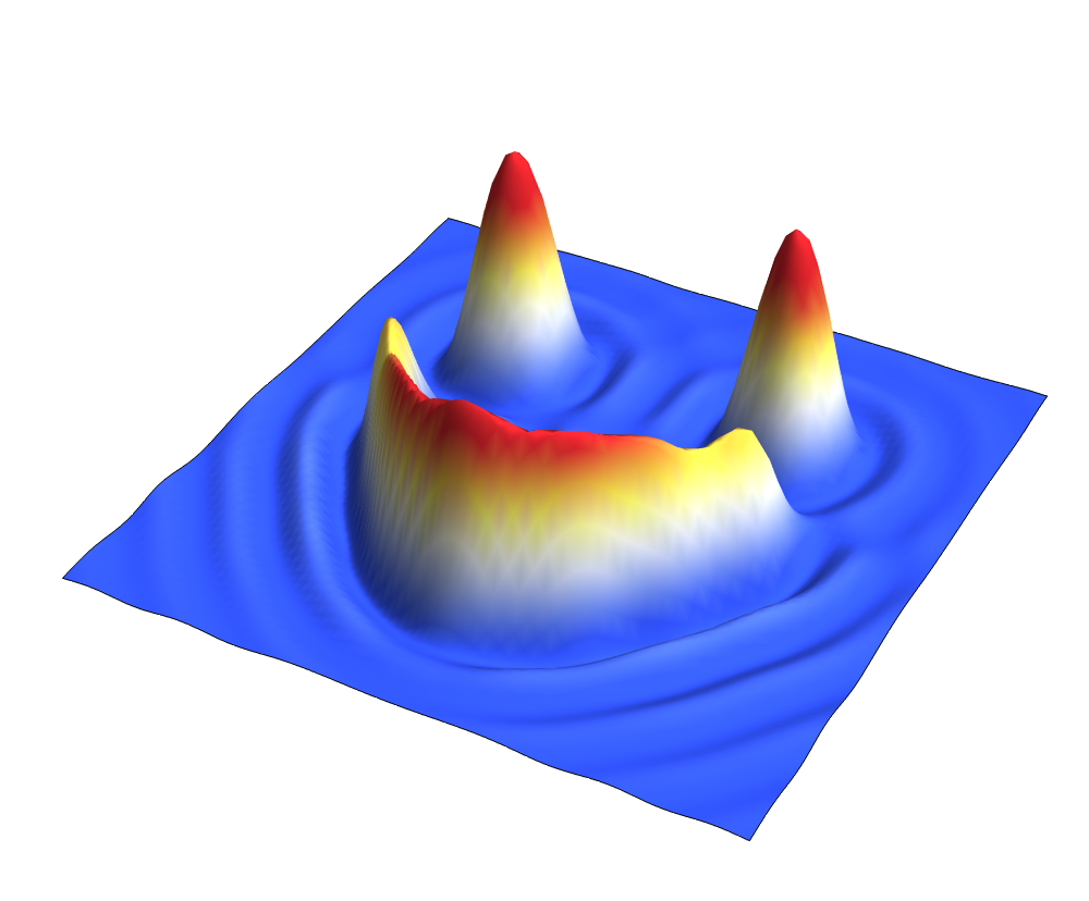
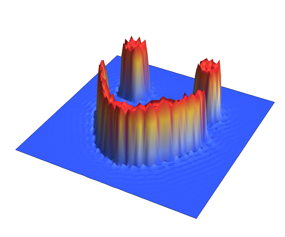
Wave equation 2D
\[\frac{\partial^2 u}{\partial t^2} = \frac{\partial^2 u}{\partial x^2} + \frac{\partial^2 u}{\partial y^2}\]
Wave equation 2D with initial speed
\[\frac{\partial^2 u}{\partial t^2} = \frac{\partial^2 u}{\partial x^2} + \frac{\partial^2 u}{\partial y^2}\]
Wave equation 2D
\[\frac{\partial^2 u}{\partial t^2} = \frac{\partial^2 u}{\partial x^2} + \frac{\partial^2 u}{\partial y^2}\]
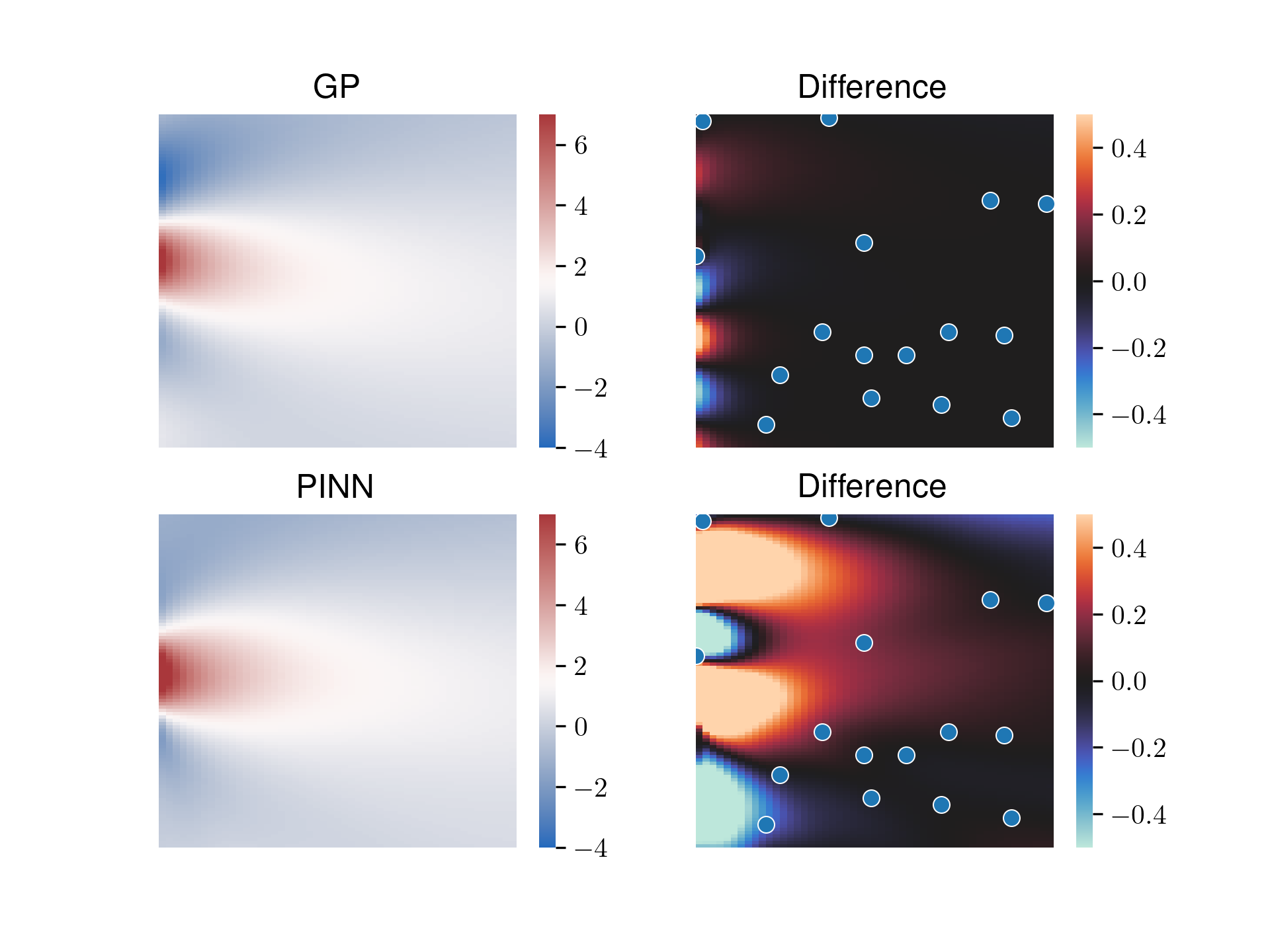
Numerical solution: Mean of our S-EPGP:
 PINN:
PINN:

First three frames of the numerical solution are the training data, with a $21\times21$ spatial grid.
Wave equation 2D
\[\frac{\partial^2 u}{\partial t^2} = \frac{\partial^2 u}{\partial x^2} + \frac{\partial^2 u}{\partial y^2}\]
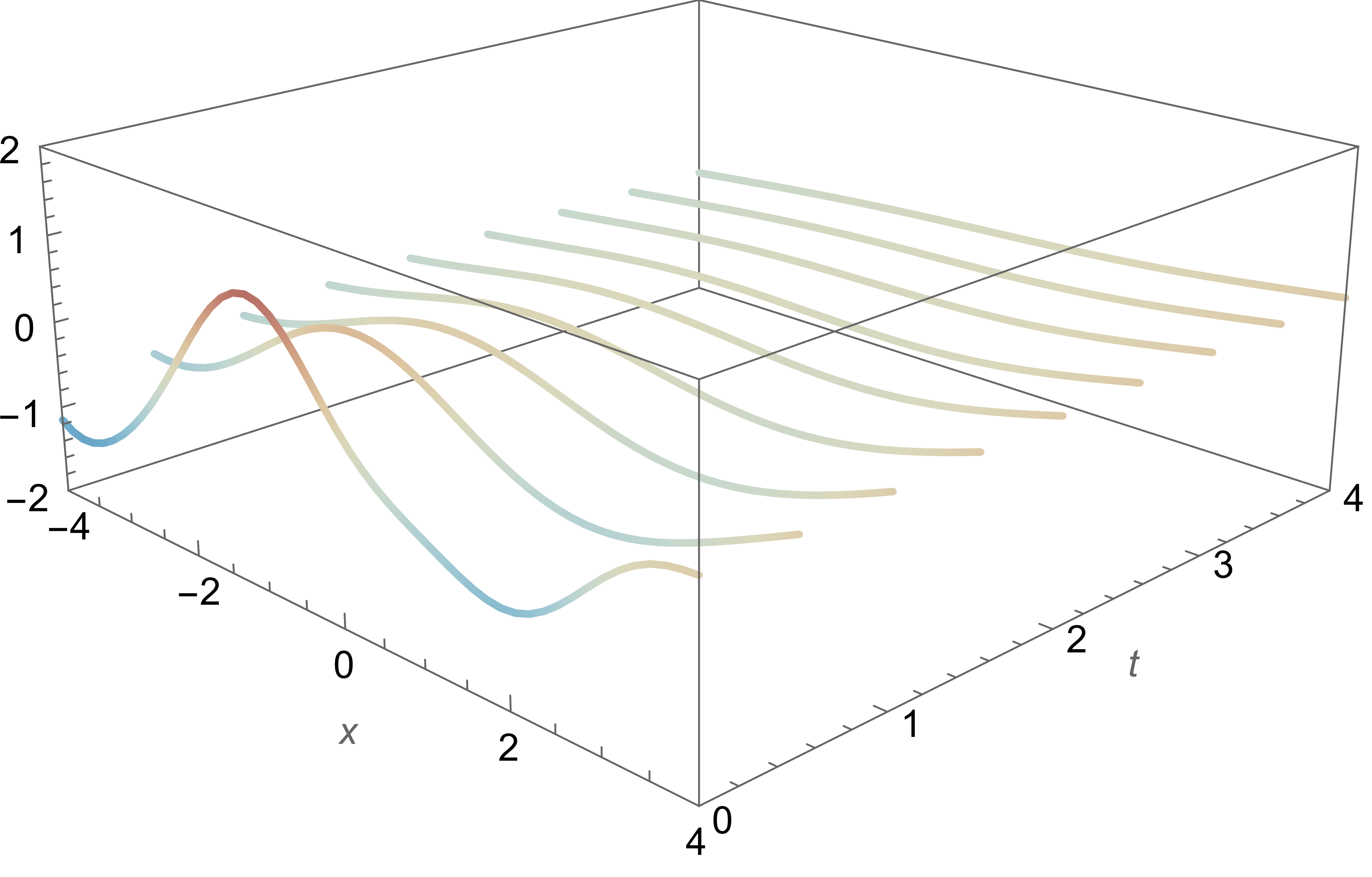
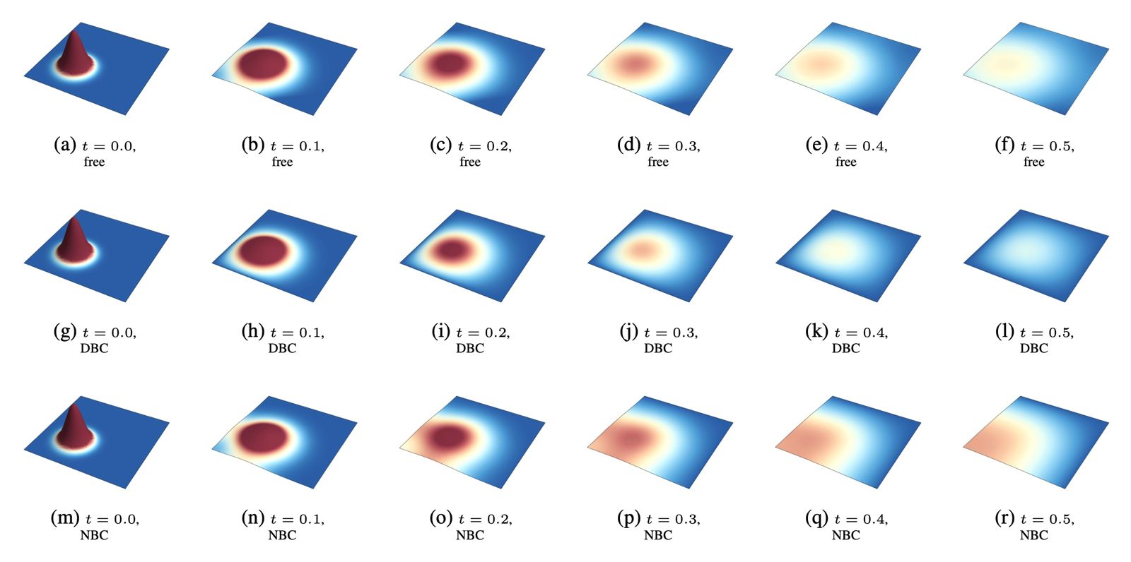
Heat Equation
Heat Equation
Heat Equation
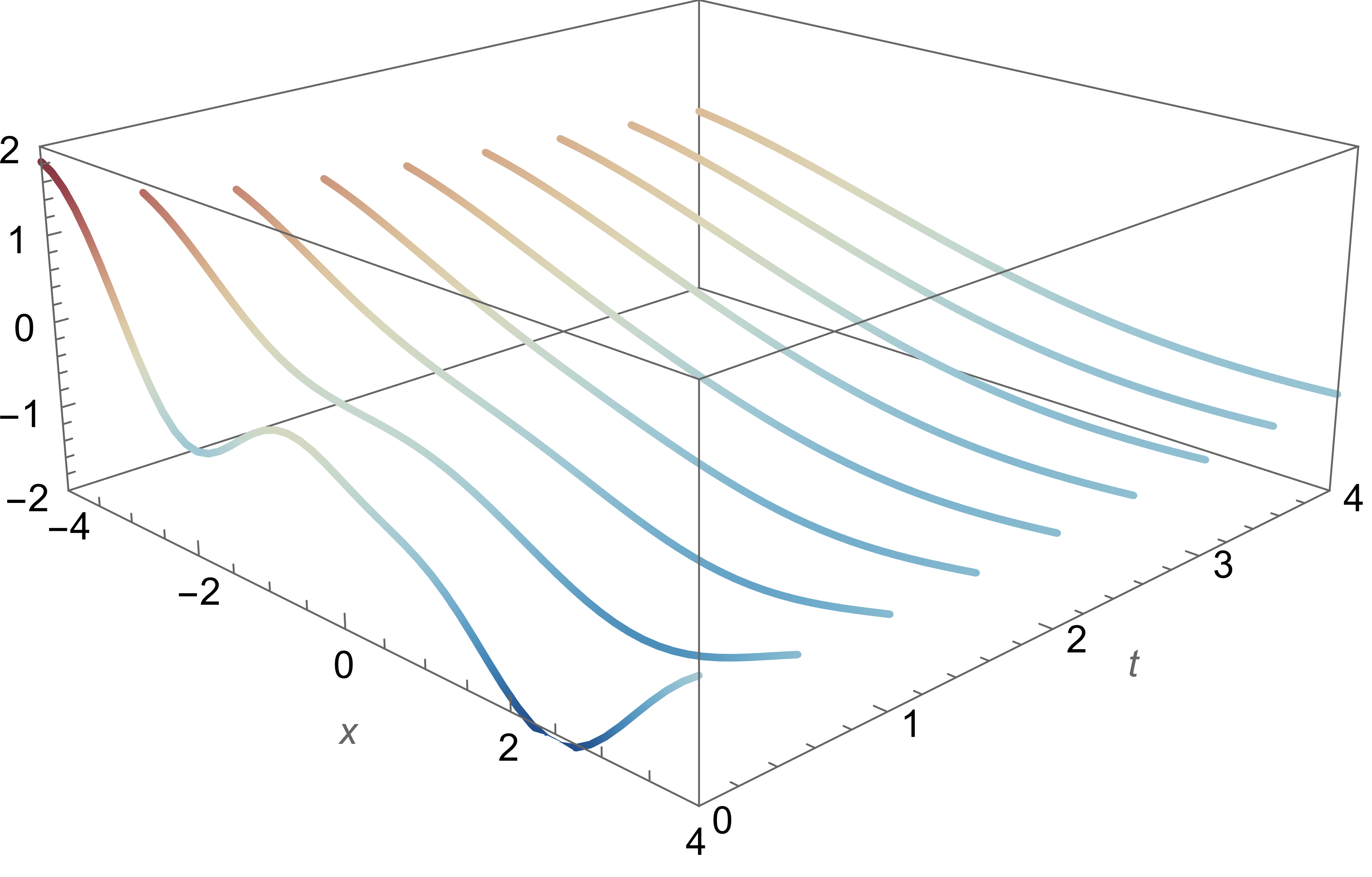
Heat Equation
Heat Equation
Heat Equation
Heat Equation
Cuomo, Di Cola, Giampaolo, Rozza, Raissi, Piccialli; Scientific machine learning through physics-informed neural networks: Where we are and what’s next. Journal of Scientific Computing; arXiv:2201.05624
Heat Equation
Maxwell's equations
\[\mathbf{E}(x,y,z,t)\]
3D wave equation
\[ \mathbf{B}(x,y,z,t) \]
Wave equation 2D
\[\frac{\partial^2 u}{\partial t^2} = \frac{\partial^2 u}{\partial x^2} + \frac{\partial^2 u}{\partial y^2}\]
Wave equation 2D
\[\frac{\partial^2 u}{\partial t^2} = \frac{\partial^2 u}{\partial x^2} + \frac{\partial^2 u}{\partial y^2}\]
Wave equation 2D
\[\frac{\partial^2 u}{\partial t^2} = \frac{\partial^2 u}{\partial x^2} + \frac{\partial^2 u}{\partial y^2}\]
Wave equation 2D
\[\frac{\partial^2 u}{\partial t^2} = \frac{\partial^2 u}{\partial x^2} + \frac{\partial^2 u}{\partial y^2}\]
Wave equation 2D
\[\frac{\partial^2 u}{\partial t^2} = \frac{\partial^2 u}{\partial x^2} + \frac{\partial^2 u}{\partial y^2}\]
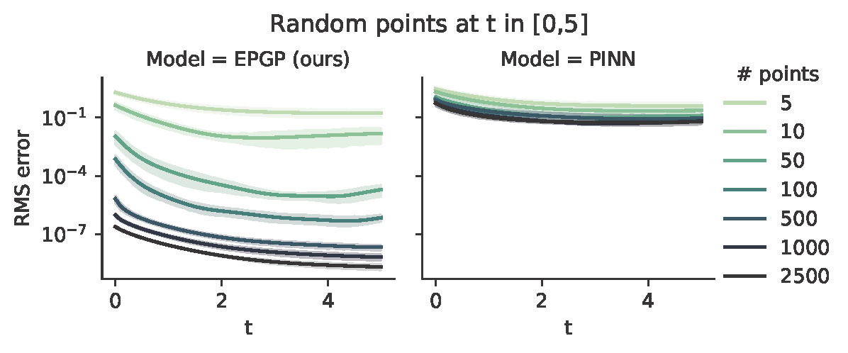
Heat equation 2D
\[\frac{\partial u}{\partial t} = \frac{\partial^2 u}{\partial x^2} + \frac{\partial^2 u}{\partial y^2}\]
Conclusion
-
EPGP: A class of GP priors for solving PDE
- S-EPGP: sparse version
- Fully algorithmic
- No approximations anywhere $\Rightarrow$ exact solutions
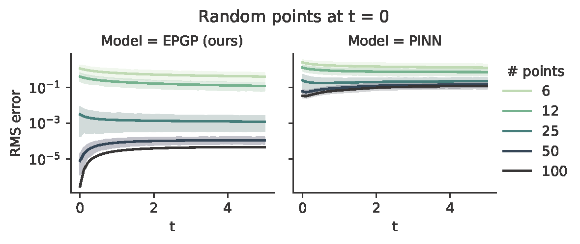
- Improved accuracy and convergence speed over PINN
- Compatible with standard GP techniques
- Interpretable hyperparameters (optimizable)
- Only assumptions: linear and constant coefficients
- Very little data necessary
- We can say more for parametrizable/controllable systems
\[ \frac{\partial^2 u}{\partial t^2} = \frac{\partial^2 u}{\partial x^2} + \frac{\partial^2 u}{\partial y^2} \]
Conclusion
\[ \frac{\partial^2 u}{\partial t^2} = \frac{\partial^2 u}{\partial x^2} + \frac{\partial^2 u}{\partial y^2} \]
Open Problems
- Many
- Large scale problems and comparison to numerical solvers
- Extensions to neural networks
- Bringing these methods to industry
- Boundary conditions for S-EPGP
- Convergence and density questions
- Topologically interesting domains and monodromy phenomena
Conclusion
Thank you for your attention!
Literature
- arXiv:2411.16663
- arXiv:2212.14319 (ICML 2023)
- arXiv:2208.12515 (NeurIPS 2022)
- arXiv:2205.03185 (CASC 2022)
- arXiv:2002.00818 (AISTATS 2021)
- arXiv:1801.09197 (NeurIPS 2018)
\[ \frac{\partial^2 u}{\partial t^2} = \frac{\partial^2 u}{\partial x^2} + \frac{\partial^2 u}{\partial y^2} \]